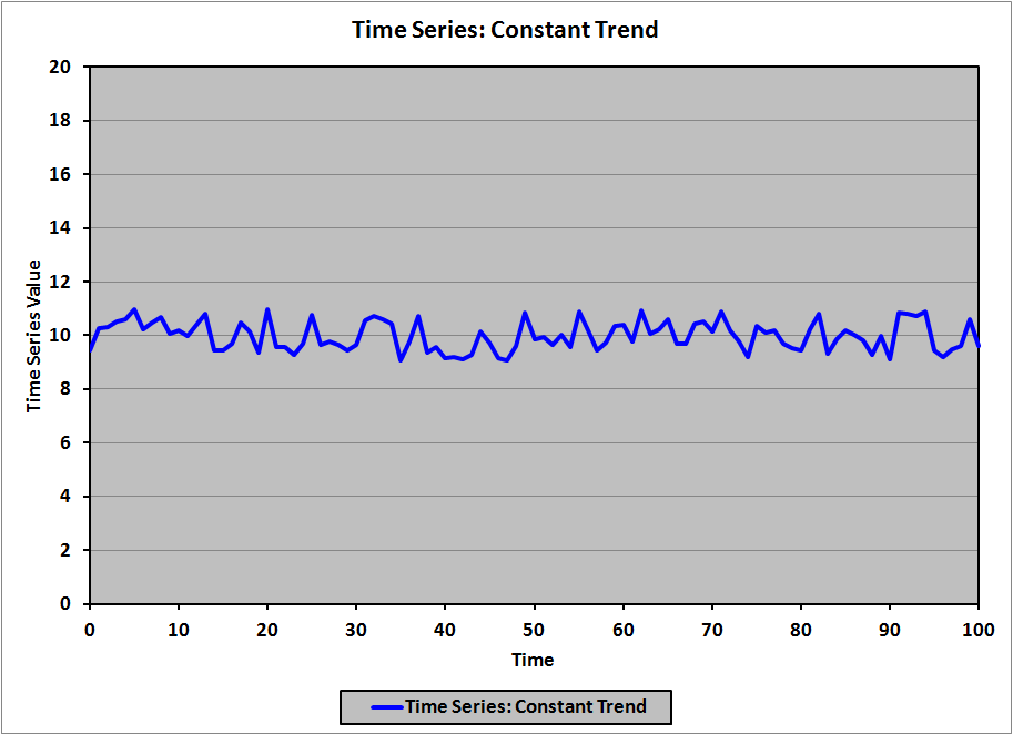
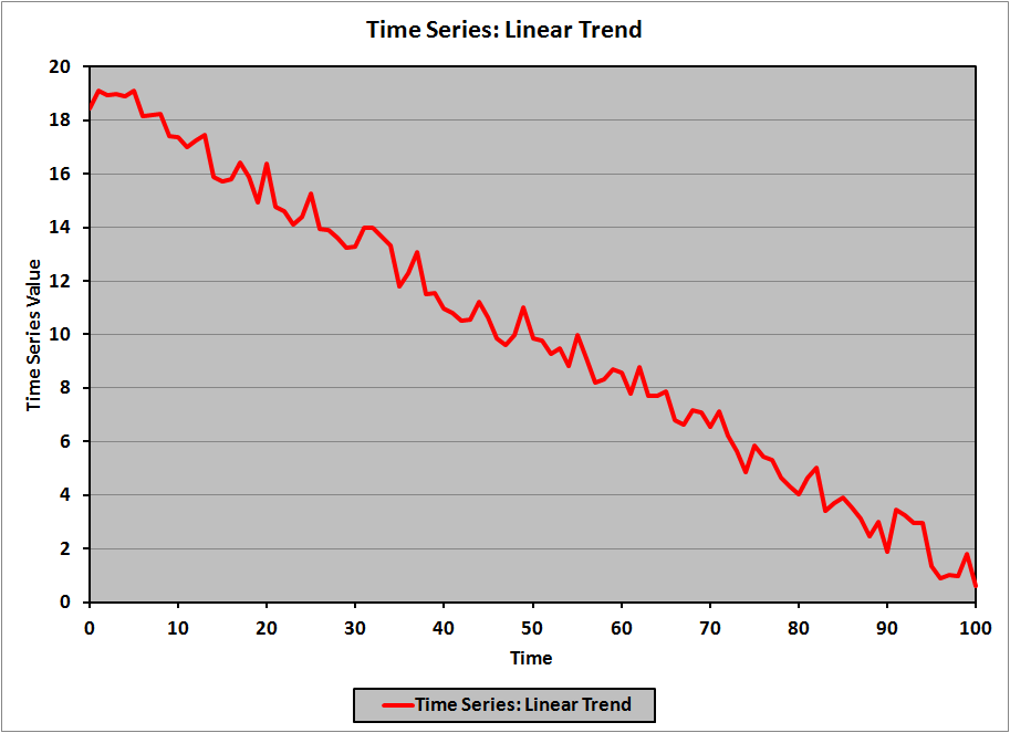
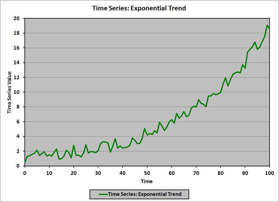
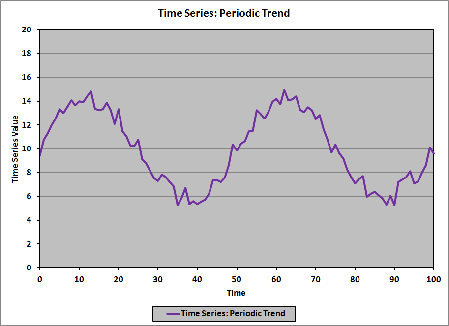
In the universe of time-series models, trend models are perhaps the easiest to understand and analyze.  A trend model is, as it turns out, exactly what its name suggests: a model of a time-dependent phenomenon that has a clear (obvious) trend to the values.  There are numerous types of trends that are possible; for example, here are illustrations of four types of trends:

• Constant
• Linear
• Exponential
• Periodic

For the Level II CFA exam, you need to know about only two of these:

• Linear trend, of which the constant trend is a special case
• Exponential trend

I’ll cover these in detail.

Linear Trend

The formula for a linear time-series model is:

\[y_t = b_0 + b_1\left(t\right) + \epsilon_t\]

where:

• \(t\): independent variable (time); \(t = 1, 2, \dots, T\)
• \(y_t\): value of the dependent variable at time \(t\)
• \(b_0\): intercept (value of \(y_t\) when \(t = 0\))
• \(b_1\): slope coefficient (also called “trend coefficient”)
• \(\epsilon_t\): error term at time \(t\)

We estimate the parameters (i.e., the intercept and the slope, b₀ and b₁, respectively) using a bunch of data we’ve gathered, and some calculus; the result is:

\[\hat{y}_t = \hat{b}_0 + \hat{b}_1\left(t\right)\]

where:

• \(\hat{y}_t\): estimated (predicted) value of the dependent variable at time \(t\)
• \(\hat{b}_0\): estimated value of the intercept parameter
• \(\hat{b}_1\): estimated value of the slope coefficient

Example

Suppose that you’re given a linear trend model with \(\hat{b}_0\) = 27.943, and \(\hat{b}_1\) = -2.135.  What are the predicted y-values for t = 5 and t = 10?

\begin{align}\hat{y}_5 &= \hat{b}_0 + \hat{b}_1\left(5\right)\\
\\
&= 27.943\ -\ 2.135\left(5\right)\\
\\
&= 17.268
\end{align}

\begin{align}\hat{y}_{10} &= \hat{b}_0 + \hat{b}_1\left(10\right)\\
\\
&= 27.943\ -\ 2.135\left(10\right)\\
\\
&= 16.593
\end{align}

If the slope coefficient b₁ = 0, then the trend is constant (as in the first  (blue) graph, above).  If b₁ > 0, then the trend is positive, and the overall graph slopes upward; and if b₁ < 0, then the trend is negative, and the overall graph slopes downward (as in the second (red) graph, above).

Exponential Trend

If a time series demonstrates exponential growth (compound growth), then the formula (without the error term; more on this later) will be:

\[y_t = e^{b_0 + b_1\left(t\right)}\]

Although it is certainly possible to create a model by fitting an exponential curve to the data, it’s more common to transform this model into a linear model, simply by taking the natural logarithm of both sides:

\begin{align}ln\left(y_t\right) &= ln\left(e^{b_0 + b_1\left(t\right)}\right)\\
\\
ln\left(y_t\right) &= b_0 + b_1\left(t\right)
\end{align}

Commonly, a time series that displays exponential growth is modeled directly using this last formula, with the error term included (rather than including the error term in the original (exponential) formula above):

\[ln\left(y_t\right) = b_0 + b_1\left(t\right) + \epsilon_t\]

We refer to this model as a log-linear model (natural logarithm on the left side, linear function on the right side).  For example, if the data in the exponential trend (green) graph, above, are transformed by taking the natural logarithm, the resulting graph is:

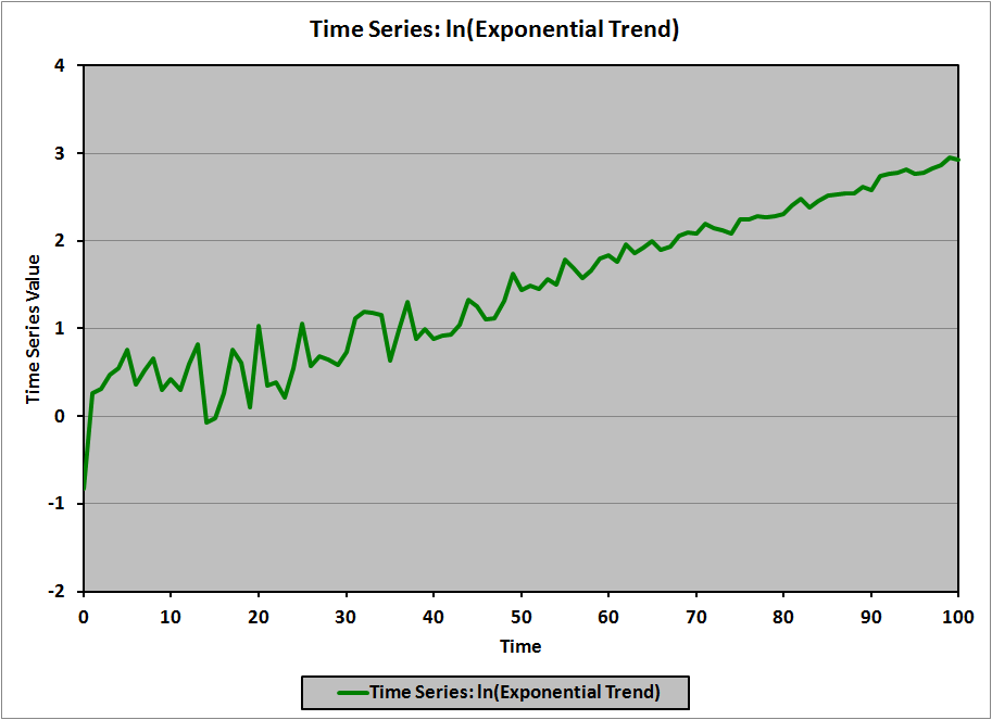
(Of note is that the error terms are of roughly constant magnitude in the original (exponential) graph (I know that they are because I created the graph), while the error terms in the transformed graph are clearly larger for small values of t, and decrease as t increases.  The CFA curriculum doesn’t address this particular example of heteroskedasticity, but I’d be quite surprised if it weren’t the subject of some common correction technique in the statistical literature.)

As with the linear model, the parameters in the log-linear model are estimated from historical data using fancy-schmancy calculus:

\[ln\left(\hat{y}_t\right) = \hat{b}_0 + \hat{b}_1\left(t\right)\]

Example

Suppose that you’re given a log-linear trend model with \(\hat{b}_0\) = 0.0116, and \(\hat{b}_1\) = 0.029.  What are the predicted y-values for t = 25 and t = 75?

\begin{align}\ln\left(\hat{y}_{25}\right) &= \hat{b}_0 + \hat{b}_1\left(25\right)\\
\\
&= 0.0116 + 0.029\left(25\right)\\
\\
&= 0.7366\\
\\
\hat{y}_{25} &= e^{0.7366}\\
\\
&= 2.0888
\end{align}

\begin{align}\ln\left(\hat{y}_{75}\right) &= \hat{b}_0 + \hat{b}_1\left(75\right)\\
\\
&= 0.0116 + 0.029\left(75\right)\\
\\
&= 2.1866\\
\\
\hat{y}_{75} &= e^{2.1866}\\
\\
&= 8.9049
\end{align}

If you’re given a log-linear model, please remember that the linear function gives you ln(y); you have to raise e to that power to get y.