In computing modified (or effective) duration for a portfolio of securities, we change the par interest rate (the yield to maturity) at every maturity by some small amount up and down (±Δy), and determine the percentage price change in the portfolio for 1% change in yield. In essence, we add ±Δy to the entire par curve. (Look here for a refresher on the par curve, and for a refresher on bootstrapping the spot curve from the par curve, which we shall be doing a bit later.) Parallel shifts in the par curve look like this:
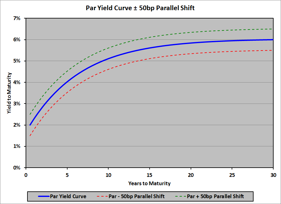
Modified (or effective) duration is useful for determining how the price of a security or a portfolio of securities will change when the (par) yield curve undergoes a parallel shift, but is less useful (i.e., not useful at all) when the yield curve changes in a manner other than a parallel shift (e.g., flattening or steepening). A more versatile measure of duration is needed in those cases; key rate duration is just such a measure.
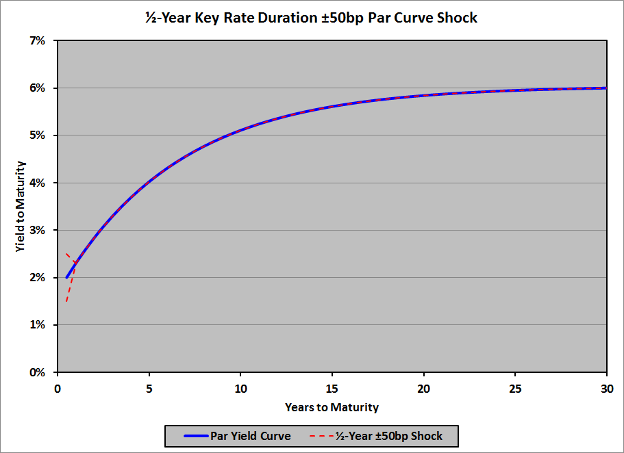
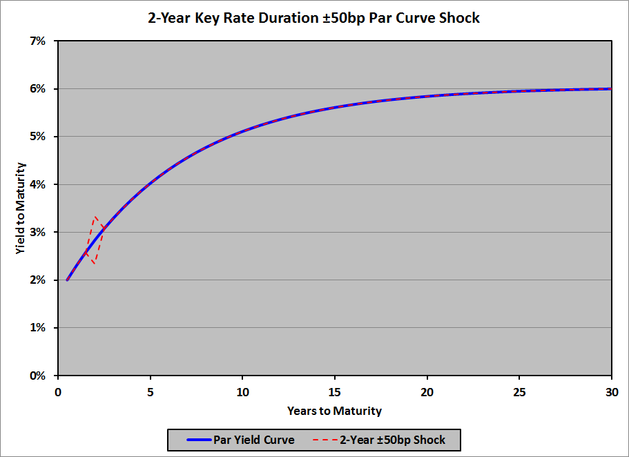
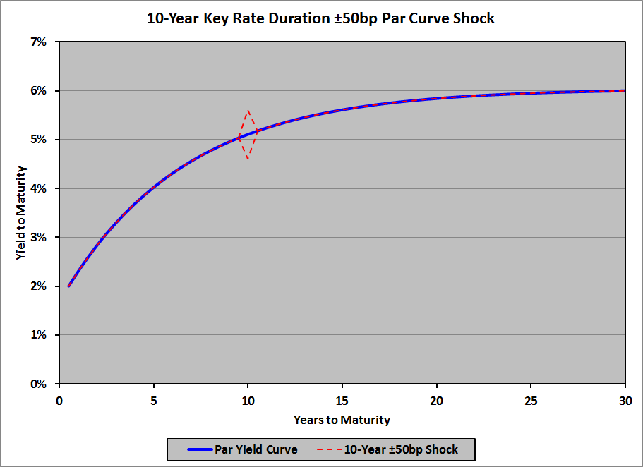
The idea of a key rate duration (also known as partial duration) is that we don’t add ±Δy to the entire par curve; we add ±Δy only to the YTM at a specific maturity on the par curve, leaving the YTM at all other maturities unchanged; that specific maturity is called the key rate. Thus, we have the:
- ½-year key rate duration: ±Δy added to the ½-year YTM, while the YTMs at all other maturities remain unchanged
- 2-year key rate duration: ±Δy added to the 2-year YTM
- 5-year key rate duration: ±Δy added to the 5-year YTM
- 10-year key rate duration: ±Δy added to the 10-year YTM
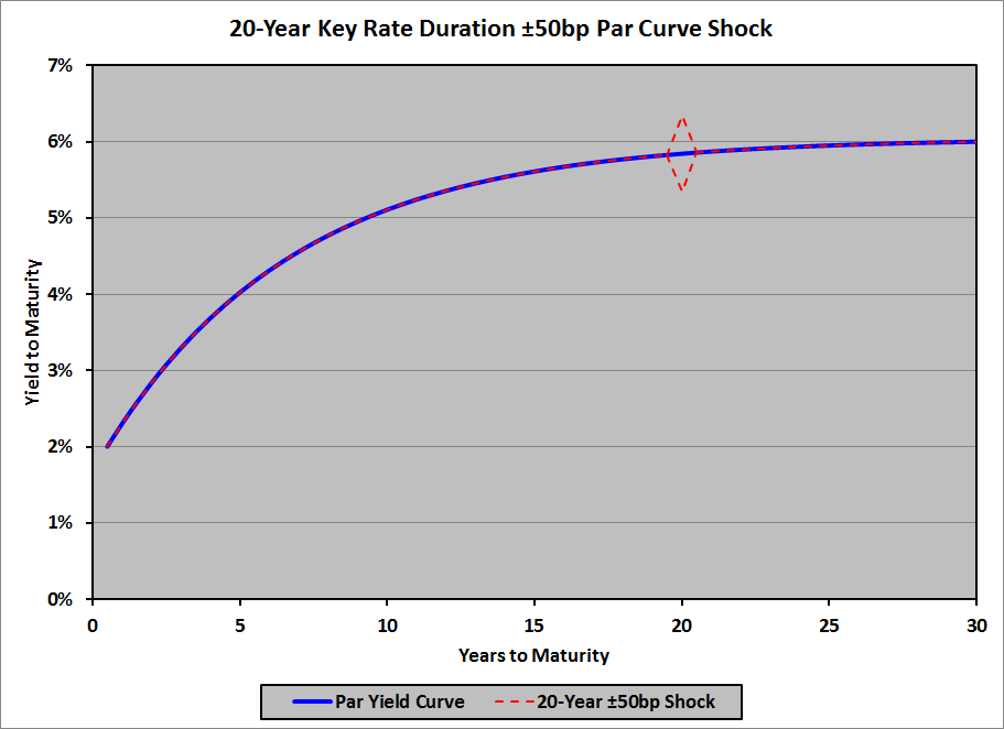
- 20-year key rate duration: ±Δy added to the 20-year YTM
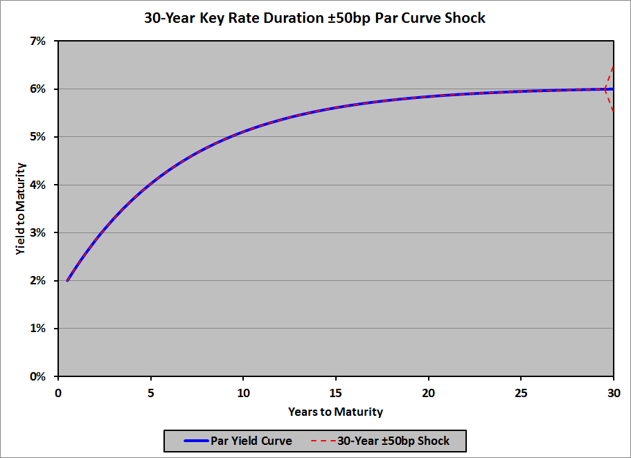
- 30-year key rate duration: ±Δy added to the 30-year YTM
- And so on
Shifts in the par curve to calculate key rate durations look like this:

Note that key rate durations can be modified (assuming no changes to the cash flows when the key rate changes) or effective (allowing that cash flows might change when the key rate changes). There’s probably no reason to concern yourself about this as far as the exam goes, but in real world applications you might as well assume that key rate durations are effective durations.
Once the effect of the key-rate shift is incorporated into the bond price, the duration is computed using the standard (modified or effective) duration formula:
\[Dur_{key\ rate}\ =\ \frac{P_–\ -\ P_+}{2P_0\Delta y}\]
In many respects, key rate durations behave exactly like all other durations (Macaulay duration, modified duration, effective duration, etc.), but in some ways their behavior is unusual. We’ll cover both.
Expected Behavior
Key Rate Duration of a Portfolio
As with Macaulay, modified, and effective duration (see here), any particular key rate duration of a portfolio is the weighted average of that particular key rate duration for each of its constituent bonds, where the weights are based on the market values of the constituent bonds:
\begin{align}Dur_{key\ rate_{port}}\ &=\ W_1\ ×\ Dur_{key\ rate_{bond\ 1}}\ +\ W_2\ ×\ Dur_{key\ rate_{bond\ 2}}\\
&+\ \cdots\ +\ W_n\ ×\ Dur_{key\ rate_{bond\ n}}\\
\\
&=\ \sum_{i=1}^n W_i\ ×\ Dur_{key\ rate_{bond\ i}}
\end{align}
where:
- \(W_i\): bond i‘s market value ÷ market value of the portfolio
So, for example, the 5-year key rate duration of a portfolio of bonds is the weighted average of the 5-year key rate durations of each of the constituent bonds, the 20-year key rate duration of the portfolio is the weighted average of the 20-year key rate durations of each of the constituent bonds, and so on.
Relationship of (Modified or Effective) Duration and Key Rate Durations
Another characteristic of key rate durations that is expected (or, at least, should be, once you think of it) is that the (modified or effective) duration of a security or a portfolio is the sum of all of its own (respectively, modified or effective) key rate durations:
\begin{align}Dur\ &=\ Dur_{key\ rate_1}\ +\ Dur_{key\ rate_2}\ +\ \cdots\ +\ Dur_{key\ rate_k}\ +\cdots\\
\\
&=\ \sum_{i=1}^{\infty}\ Dur_{key\ rate_i}
\end{align}
Note that this is not an infinite sum: eventually the index i will exceed the maturity of the security or portfolio; after that, all of the key rate durations will be zero (because, as we will see, all of the par rates and all of the spot rates at maturities shorter than the key rate maturity are unchanged).
Unusual Behavior
Recalling the link between the par curve and the spot curve, we can determine the effect of key rate changes on bonds of various maturities and with various coupons. To illustrate these effects, I’ll use a simple example: a 4% flat yield curve with annual (effective) rates from 1 year to 10 years:
| Maturity (Years) |
Par Yield |
Spot Yield |
| 1.0 |
4.0% |
4.0% |
| 2.0 |
4.0% |
4.0% |
| 3.0 |
4.0% |
4.0% |
| 4.0 |
4.0% |
4.0% |
| 5.0 |
4.0% |
4.0% |
| 6.0 |
4.0% |
4.0% |
| 7.0 |
4.0% |
4.0% |
| 8.0 |
4.0% |
4.0% |
| 9.0 |
4.0% |
4.0% |
| 10.0 |
4.0% |
4.0% |
Suppose that we want to compute the 5-year key rate duration of a bond. To do this, we add 50bp to the 5-year par rate (leaving all of the other par rates unchanged), and compute the effect on the spot rates, then subtract 50bp from the 5-year par rate (again, leaving all of the other par rates unchanged), and compute the effect on the spot rates. We’ll then use those modified spot rates to compute \(P_-\) and \(P_+\), and then use them in the duration formula.
Let’s start by adding 50bp to the 5-year par rate, leaving all other par rates unchanged at 4.0%.
The first question is: what happens to the 1-year spot yield? The answer is easy: it remains 4.0%. (Recall that the one-period par rate and the one-period spot rate are equal, and that the 1-year par rate hasn’t changed; only the 5-year par rate has changed.)
The 2-year spot yield is also easy: it, too, remains 4.0%, because the 2-year par yield is unchanged, and the 1-year spot yield is unchanged. If you want to run through the algebra, it’s:
\begin{align}$1,000\ &=\ \frac{$40.00}{1.04}\ +\ \frac{$1,040.00}{\left(1\ +\ s_2\right)^2}\\
\\
$1,000\ &=\ $38.46\ +\ \frac{$1,040.00}{\left(1\ +\ s_2\right)^2}\\
\\
$961.54\ &=\ \frac{$1,040.00}{\left(1\ +\ s_2\right)^2}\\
\\
\left(1\ +\ s_2\right)^2\ &=\ \frac{$1,040.00}{$961.54}\ =\ 1.0816\\
\\
1\ +\ s_2\ &=\ \sqrt{1.0816}\ =\ 1.0400\\
\\
s_2\ &=\ 4.0\%
\end{align}
The 3-year spot rate and the 4-year spot rate are also easy: they’re both still 4.0%, because their par yields are unchanged, as are all of the spot yields for shorter maturities. I’ll leave the algebra to you.
As an exciting (!) change of pace, the 5-year spot rate isn’t 4.0% (recall that we’ve added 50bp to the 5-year par rate). A 5-year bond paying a 4.5% (= 4.0% + 50bp) will therefore sell at par, so:
\begin{align}$1,000\ &=\ \frac{$45.00}{1\ +\ s_1}\ +\ \frac{$45.00}{\left(1\ +\ s_2\right)^2}\ +\ \frac{$45.00}{\left(1\ +\ s_3\right)^3}\ +\ \frac{$45.00}{\left(1\ +\ s_4\right)^4}\ +\ \frac{$1,045.00}{\left(1\ +\ s_5\right)^5}\\
\\
&=\ \frac{$45.00}{1.04}\ +\ \frac{$45.00}{1.04^2}\ +\ \frac{$45.00}{1.04^3}\ +\ \frac{$45.00}{1.04^4}\ +\ \frac{$1,045.00}{\left(1\ +\ s_5\right)^5}\\
\\
$1,000\ &=\ $43.27\ +\ $41.61\ +\ $40.00\ +\ $38.47\ +\ \frac{$1,045.00}{\left(1\ +\ s_5\right)^5}\\
\\
$836.65\ &=\ \frac{$1,045.00}{\left(1\ +\ s_5\right)^5}\\
\\
\left(1\ +\ s_5\right)^5\ &=\ \frac{$1,045.00}{$836.65}\ =\ 1.249022\\
\\
1\ +\ s_5\ &=\ 1.249022^{1/5}\ =\ 1.045476\\
\\
s_5\ &=\ 4.5476\%
\end{align}
This result seems reasonable: the YTM is 4.5%, so we’ll get par ($1,000) if we discount all of the cash flows at 4.5%. Because we’ve discounted the first four payments at 4% (less than 4.5%), we have to discount the final payment at more than 4.5% to average a 4.5% discount for everything. And because the first four payments are much smaller than the final payment, the difference on the final discount rate should be much smaller than the (50bp) difference on the first four: it’s 4.76bp.
Now comes the really interesting part (!!): the 6-year spot rate. Let’s do the algebra (recalling that the 6-year par rate hasn’t changed: it’s still 4.0%):
\begin{align}$1,000\ &=\ \frac{$40.00}{1.04}\ +\ \frac{$40.00}{1.04^2}\ +\ \frac{$40.00}{1.04^3}\ +\ \frac{$40.00}{1.04^4}\\
\\
&+\ \frac{$40.00}{1.045476^5}\ +\ \frac{$1,040.00}{\left(1\ +\ s_6\right)^6}\\
\\
$1,000\ &=\ $38.46\ +\ $36.98\ +\ $35.56\ +\ $34.19\ +\ $32.03\ +\ \frac{$1,040.00}{\left(1\ +\ s_6\right)^6}\\
\\
$822.78\ &=\ \frac{$1,040.00}{\left(1\ +\ s_6\right)^6}\\
\\
\left(1\ +\ s_6\right)^6\ &=\ \frac{$1,040.00}{$822.78}\ =\ 1.264009\\
\\
1\ +\ s_6\ &=\ 1.264009^{1/6}\ =\ 1.039820\\
\\
s_6\ &=\ 3.9820\%
\end{align}
Again, this result makes sense: the 5-year spot rate has increased, so the only way that the 6-year par rate can remain unchanged is for the 6-year spot rate to decrease. And, once again, because the final payment is much larger than the first 5 (coupon only) payments, the decrease should be small compared to the increase in the 5-year spot rate: the 5-year spot rate is 54.76bp higher than the 4% YTM, while the 6-year spot rate is 1.80bp lower than the YTM.
Note how the change in the 5-year key rate leads to some somewhat surprising results. For example, a 6-year zero-coupon bond will have a slightly higher price (because the 6-year spot rate is lower) when the 5-year key rate is increased; in other words, a 6-year zero-coupon bond will have a negative 5-year key rate duration. (Remember that when interest rates increase, bond prices normally decrease, and that duration is normally positive. When the price increases with a rate increase, duration must be negative.)
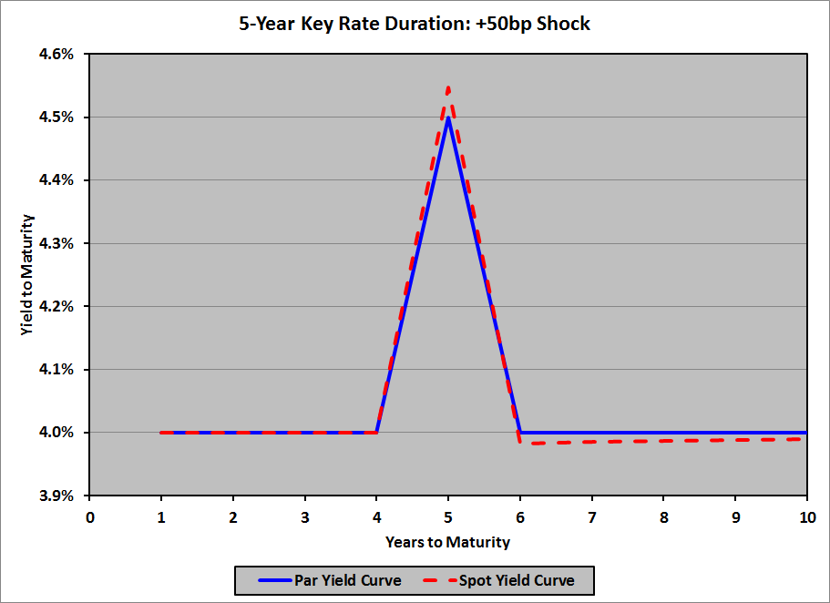
Continuing in this same tedious manner, we get:
| Maturity (Years) |
Par Yield |
Spot Yield |
| 1.0 |
4.0000% |
4.0000% |
| 2.0 |
4.0000% |
4.0000% |
| 3.0 |
4.0000% |
4.0000% |
| 4.0 |
4.0000% |
4.0000% |
| 5.0 |
4.5000% |
4.5476% |
| 6.0 |
4.0000% |
3.9820% |
| 7.0 |
4.0000% |
3.9846% |
| 8.0 |
4.0000% |
3.9865% |
| 9.0 |
4.0000% |
3.9880% |
| 10.0 |
4.0000% |
3.9892% |
Graphically:
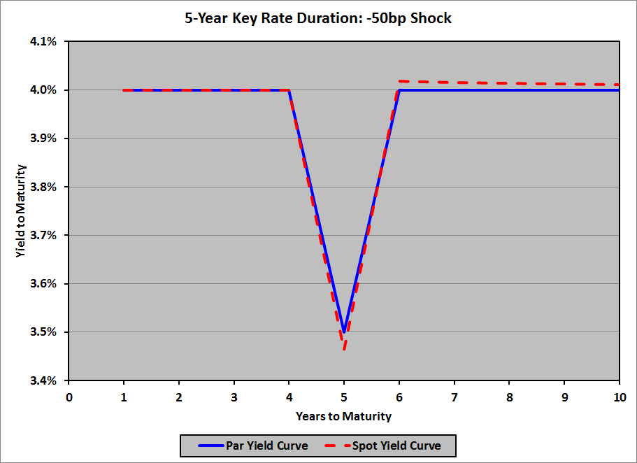
When we subtract 50bp from the 5-year par rate, we get:
| Maturity (Years) |
Par Yield |
Spot Yield |
| 1.0 |
4.0000% |
4.0000% |
| 2.0 |
4.0000% |
4.0000% |
| 3.0 |
4.0000% |
4.0000% |
| 4.0 |
4.0000% |
4.0000% |
| 5.0 |
3.5000% |
3.4641% |
| 6.0 |
4.0000% |
4.0182% |
| 7.0 |
4.0000% |
4.0156% |
| 8.0 |
4.0000% |
4.0136% |
| 9.0 |
4.0000% |
4.0121% |
| 10.0 |
4.0000% |
4.0109% |
Graphically:
Key Rate Durations of Various Bonds
Not only does the key rate duration of a bond depend on the bond’s maturity (compared to the maturity of the key rate), it also depends on the bond’s coupon rate compared to its YTM; i.e., it depends on whether the bond is priced at par, at a premium, or at a discount. Using our 4% flat yield curve, here are the key rate durations for five 5-year, option-free bonds with varying coupon rates, along with the sum of their key rate durations, and their effective durations:
| Key Rate Duration (Years), 5-Year Bond |
| Key Rate Maturity |
Coupon Rate |
| 0.0% |
2.0% |
4.0% |
6.0% |
8.0% |
| 1 Year |
(0.0385) |
(0.0174) |
0.0000 |
0.0145 |
0.0268 |
| 2 Years |
(0.0785) |
(0.0354) |
0.0000 |
0.0296 |
0.0547 |
| 3 Years |
(0.1201) |
(0.0542) |
0.0000 |
0.0453 |
0.0838 |
| 4 Years |
(0.1633) |
(0.0737) |
0.0000 |
0.0616 |
0.1140 |
| 5 Years |
5.2081 |
4.7931 |
4.4519 |
4.1666 |
3.9243 |
| 6+ Years |
0.0000 |
0.0000 |
0.0000 |
0.0000 |
0.0000 |
| Sum |
4.8078 |
4.6125 |
4.4519 |
4.3176 |
4.2036 |
| DurEff |
4.8078 |
4.6125 |
4.4519 |
4.3176 |
4.2036 |
So, for example, a 5-year, zero-coupon bond has a 4-year key rate duration of −0.1633 years; if the 4-year par rate increases by 1%, the price of the bond will increase by approximately 0.1633%. A 5-year, 8% coupon bond has a 3-year key rate duration of 0.0838 years; if the 3-year par rate decreases by 1%, the price of the bond will increase by approximately 0.0838%.
The key ideas to glean from this table are:
- Par bonds have key rate durations of zero years for any key rate maturity shorter than the bond’s maturity
- Discount bonds have negative key rate durations for key rate maturities shorter than the bond’s maturity; in particular, zero-coupon bonds have negative key rate durations for key rate maturities shorter than the bond’s maturity
- Premium bonds have positive key rate durations for key rate maturities shorter than the bond’s maturity
- All bonds have key rate durations of zero years for any key rate maturity longer than the bond’s maturity
- The sum of the key rate durations for all key rate maturities equals the bond’s effective duration
Note that these last two points was already covered under Expected Behavior, above.
Using Key Rate Durations
Key rate durations are used to determine the effect of non-parallel yield curve shifts on a portfolio of bonds. (In fact, they can also be used to determine the effect of parallel yield curve shifts, although they’re less efficient than simply using the effective duration of each bond.) For example, suppose that we have this par yield curve:
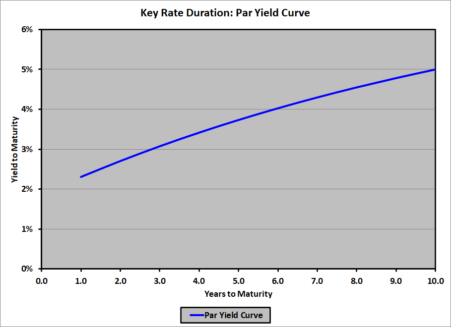
Suppose that we expect the yield curve to flatten: rise 50bp on the short end, fall 50bp on the long end, with a linear transition in between:
| Years |
Flattening ∆, bp |
| 1.0 |
50.0 |
| 2.0 |
38.9 |
| 3.0 |
27.8 |
| 4.0 |
16.7 |
| 5.0 |
5.6 |
| 6.0 |
−5.6 |
| 7.0 |
−16.7 |
| 8.0 |
−27.8 |
| 9.0 |
−38.9 |
| 10.0 |
−50.0 |
The new (par) yield curve will look like this:
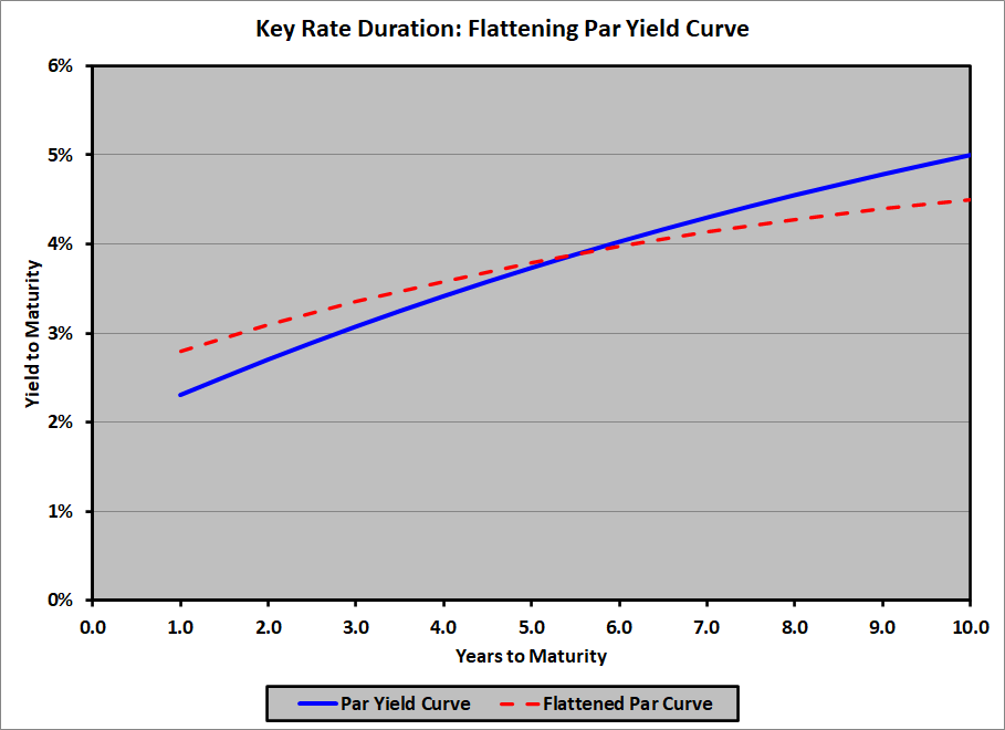
To determine the effect of this flattening on the value of a fixed income portfolio, we can look at the key-rate durations of each bond in the portfolio, multiply each key rate duration by the yield change (from the table, above) and the bond’s market value, then tot them up. Note that effective duration (of the portfolio) will not help here, as the shift is not parallel.
Similarly, if we expect the par curve to steepen, or hump, or do anything else other than a parallel shift, key rate durations will allow us to determine the first-order effect on the value of a portfolio of bonds with a range of maturities.
For whatever it’s worth, there’s also the idea of key rate convexities. I’ve never heard of them – I just came up with the idea all on my own – but for large yield changes it would make sense to consider convexity in addition to duration. Deep down, I’m a pioneer.
Misconceptions about Key Rate Durations
The primary misconception about key rate durations is that they correspond to a change in a single spot rate, instead of a change in a single par rate. To be clear:
- The key rate duration of a given bond for a given maturity is the ratio of the percentage change in that bond’s price to the change in the par rate at that maturity, when the par rates at all other maturities remain unchanged.
- When the par rate at a given maturity changes, and the par rates at all other maturities remain unchanged:
- The spot rates at maturities less than the given maturity will not change
- The spot rate at the given maturity will change in the same direction as change in the par rate, and by an amount greater than the change in the par rate
- The spot rates at maturities greater than the given maturity will change in the opposite direction of the change in the par rate, and by an amount (much) less than the change in the par rate (and the change will be smaller at longer maturities)